


INTRODUCTION
Resting metabolic rate (RMR) is the total number of calories burned when the body is completely at rest. It is proportional to the lean body mass and decreases by approximately 0.01 kcal/min for each 1% increase in the body fat1. The total energy expenditure in 24 hours consists of RMR, physical activity energy expenditure (PEE), and diet-induced thermogenesis (DIT). The RMR represents approximately 60-75% of daily energy expenditure (DEE) in a 70 kg person2,3, accounting for the largest contribution to the 24-hour energy expenditure. It consequently has a large impact on the regulation of body composition and energy balance. An abnormally high RMR is associated with pathologic and inflammatory conditions. It also tends to decrease with aging, with a low RMR playing an important role in the pathogenesis of obesity and age related chronic diseases4-6. Therefore, an accurate measurement of the RMR is very important.
Methods for measuring the RMR include direct and indirect calorimetry, with the latter being used commonly due to a more efficient measurement. It is further divided into two methods, one using doubly labeled water; and the other using a human metabolic chamber, a hood-, or a mask system7-9. However, both the methods require tedious procedures and are time- and cost- consuming. Thus, many researchers have developed various regression models for RMR estimation2,9-14. Determining the contribution of the RMR to the DEE is an important calculation for understanding, developing, and executing body weight- related interventions3,4. For example, RMR estimation regression model is applied to determine the target energy intake in weight loss programs, develop dynamic prediction models of weight gain and loss, identify the patients with potential metabolic abnormalities, design public health programs promoting obesity prevention in diverse populations, and assess the potential energy deficits in metabolically stressed patients4.
The previous regression models were developed using only height, age, weight, and fat-free mass (FFM) and hence did not have a high correlation and regression rate. The Harris-Benedict regression model10 was the most commonly used, but only 50-75% of the RMR variability could be explained by this equation. Its major disadvantage was overestimating RMR by at least 5%. Additionally, RMR was estimated only by age, height, and weight and the regression rate, R2 value, did not exceed 0.7. Previous attempts to overcome these shortcomings failed to show high regression rates11-14, as they also estimated RMR with only age, height, weight, and lean body mass. Therefore, developing a regression model, with a higher regression rate using various dependent variables, is important for accurate RMR measurements.
The present study was a preliminary study and it aimed to evaluate the Korean adults (males and females) to generate regression equations to predict the RMR from age, height, body mass index (BMI), FFM, fat mass, % body fat, systolic blood pressure (SBP), diastolic blood pressure (DBP), mean arterial pressure (MAP), pulse pressure (PP) and resting heart rate (HR).
METHODS
Subjects
Fifty three young (males = 18, females = 16) and middle-aged (males = 5, females = 14) healthy adults were included in the present study <Table 1>7. All subjects were of Korean origin, with a stable weight for at least 3 months prior to the measurements, and without a history of thyroid disease, diabetes mellitus-I or II, cardiovascular disease, or severe hypertension in the past 6 months. There was also no history of orthopedic disease or other medical issues over the past year in the pre-screening surveys. All the subjects received a medical clearance for their participation and were explained about the purpose, procedures, and potential risks of the study. All proceedings of the study were approved by the Institutional Review Board of Konkuk University (7001355-201903-HR-305) in Korea and were conducted according to the Declaration of Helsinki. All subjects arrived at the laboratory early in the morning (8:00 AM) after overnight fasting (≥ 8 hour) and rested for 30 minutes, after which their blood pressure, body composition, and resting HR was measured, followed by the RMR measurement. All the subjects were instructed to sleep for at least 8 hours before the RMR measurement and to stay awake during the process. If they fell asleep, their shoes or toes were squeezed to keep them awake.
Table 1.
Characteristics of subjects.
Height and body composition
Height, BMI, body weight, FFM, fat mass, and % body fat were measured using the bioelectrical impedance analysis equipment (Inbody 770, Inbody, Seoul, Korea). All subjects fasted overnight prior to body composition measurement. The subjects wore lightweight clothing and were asked to remove any metal items.
Blood pressure and resting heart rate
After all the subjects were sufficiently rested for more than 20 min, their blood pressure was measured twice using an autonomic blood pressure monitor (HBP-9020, Omron, Tokyo, Japan) and the average value was used for analysis. The blood pressure parameters measured were SBP, DBP, MAP, and PP. The resting HR was measured using an autonomic HR monitor (V800, Polar, Helsinki, Finland).
Resting metabolic rate
All subjects fasted overnight, prior to the measurement of the RMR by indirect calorimetry using a metabolic gas analyzer (Quark CPET, Cosmed, Rome, Italy) with a flow-dilution canopy hood system. Calibration was performed using the calibration gas (16% O2 and 5% CO2) before the measurement. All the RMR testing procedures were performed in a 9 m (width) × 7 m (length) × 3 m (height) chamber with a temperature of 23 ± 1 °C and a humidity of 50 ± 5%, regulated by the environmental control chamber (NCTC-1, Nara Controls, Seoul, Korea). Subjects were asked to limit their physical activity and abstain from alcohol intake one day before the measurement. The subjects took a rest for 30 min, prior to the measurement. The RMR was measured in a supine position for 30 min, and the average value of the last 25 min was used for the analysis.
Statistical Analysis
The means and standard deviations were calculated for all the measured parameters. The Shapiro-Wilk test verified the normal distribution of all the outcome variables. To perform the linear regression analysis, we verified the independent variables by checking the regression coefficient (β-value). Regression analysis using the stepwise method was used to predict the RMR from age, height, BMI, FFM, fat mass, % body fat, SBP, DBP, MAP, PP, and HR. A two-tailed student’s paired t-test was used to detect differences between measured and predicted RMR. Bias was calculated as the difference between measured and predicted RMR. The authors rigorously conformed to the basic assumptions of a regression model (linearity, independency, continuity, normality, homoscedasticity, autocorrelation, and outlier). Statistical Package for the Social Sciences (SPSS) version 24.0 (IBM Corporation, Armonk, NY, USA) was used for the statistical analysis and the level of significance (p value) was set at 0.05.
RESULTS
Check outlier data
We verified the absolute value of the standardized residual as ≥ 3 to delete the outlier data. There was no outlier data in the RMR prediction model. The correlation between the measured RMR and dependent variables is shown in Table 2. We estimated the regression model using the stepwise method.
Table 2.
Correlation between dependent variables and measured RMR for estimating regression model.
| RMR (kcal/day) | ||||
|---|---|---|---|---|
|
Both (n=53) |
Males (n=23) |
Females (n=30) |
||
|
Age (yrs) |
Correlation p-value |
-.284* .039 |
-.214 .327 |
-.212 .262 |
|
Body height (cm) |
Correlation p-value |
735* .000 |
.171 .434 |
.200 .289 |
|
Body weight (kg) |
Correlation p-value |
.743* .000 |
.293 .176 |
-.065 .732 |
|
Body mass index (kg/m2) |
Correlation p-value |
.536* .000 |
.275 .204 |
-.231 .218 |
|
Fat-free mass (kg) |
Correlation p-value |
.817* .000 |
.292 .176 |
.168 .375 |
|
Fat mass (kg) |
Correlation p-value |
-.191 .171 |
.142 .517 |
-.233 .215 |
|
Percent body fat (%) |
Correlation p-value |
-.631* .000 |
.036 .870 |
-.259 .167 |
|
Systolic blood pressure (mmHg) |
Correlation p-value |
.408* .002 |
.236 .278 |
-.250 .183 |
|
Diastolic blood pressure (mmHg) |
Correlation p-value |
.279* .043 |
.295 .172 |
-.220 .242 |
|
Mean arterial pressure (mmHg) |
Correlation p-value |
.346* .011 |
.292 .176 |
-.246 .191 |
|
Pulse pressure (mmHg) |
Correlation p-value |
.277* .045 |
-.099 .653 |
-.097 .610 |
|
Heart rate (beat/min) |
Correlation p-value |
-.149 .288 |
.004 .986 |
-.060 .751 |
Significance of regression models and the independent variables
We verified the significance of each model using the F-test; and used the t-test to verify the significance of the regression coefficients of the independent variables.
Individual regression models for males and females could not be developed. This was due to the small sample size and the absence of a significant correlation between the dependent variables and the RMR which resulted in multicollinearity among all the dependent variables.
The regression coefficient of the selected independent variables (age and FFM) was statistically significant <Table 3> when an integrated regression model using the stepwise method for both males and females was developed.
Table 3.
Significance level of the regression coefficient of the independent variable (age and FFM) for each estimated regression model.
| Regression model | ||||
|---|---|---|---|---|
| Model | F-value | p-value | t-value | p-value |
|
RMR1 = 24.383 × FFM + 634.310 |
102.005 | .000* |
10.100 (FFM) |
.000* (FFM) |
|
RMR2 = 23.691 × FFM - 5.745 × age + 852.341 |
58.332 | .000* |
10.160 (FFM) |
.000* (FFM) |
|
-2.357 (age) |
.022* (age) |
|||
Performance evaluation of regression models and regression equations
The coefficients of determination (R2), adjusted coefficients of determination (adjusted R2), and standard errors of estimates (SEE) were calculated for the regression model. The mean explanatory power of RMR1 regression models estimated only by FFM was 66.7% (R2) and 66.0% (adjusted R2), while the mean SEE was 219.85 kcal/day <Table 4>. The mean explanatory power of RMR2 regression models developed by FFM and age were 70.0% (R2) and 68.8% (adjusted R2), while the mean SEE was 210.64 kcal/day <Table 4>.
Difference between measured and predicted RMR of young and middle-aged Korean adults
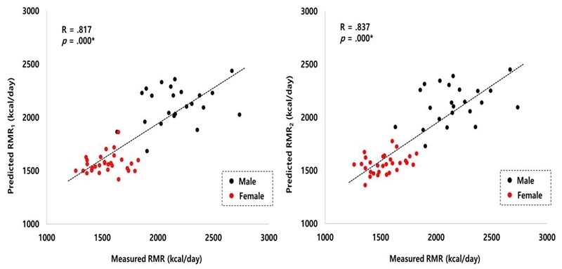
In the present study, there was no significant difference between the measured RMR by canopy method, using a metabolic gas analyzer, and the predicted RMR by RMR1 and RMR2 equations. The mean bias between the measured RMR and the predicted RMR1 and RMR2 equations was + 0.02 kcal/day and -0.01 kcal/day, respectively <Table 5>. The measured and the predicted RMR showed a similar average value, and their correlation coefficients also showed a significant correlation (measured RMR and predicted RMR1: R = 0.817, p = 0.000, measured RMR and predicted RMR2: R = 0.837, p = 0.000) <Figure 1>.
Table 5.
Measured and predicted RMR of young and middle-aged Koreans.
DISCUSSION
A preliminary study was conducted to develop a regression model for estimating the RMR of healthy young and middle-aged Korean adults using various easy-to-measure dependent variables. Based on the data obtained, our study developed two regression models (RMR1 = 24.383 × FFM + 634.310, RMR2 = 23.691 × FFM - 5.745 × age + 852.341).
Before developing a regression model to estimate the RMR, it is important to eliminate the outliers as they increase the forecast errors. In a regression analysis, the determination of outliers uses the absolute value of the standardized residual15. No outliers were observed in this study. This finding demonstrated a clear linearity between the independent and the dependent variables.
Table 2 shows the correlation between the RMR and the various dependent variables in males, females, and the total sample. Most of the measured variables presented a significant correlation with the RMR (e.g. age, height, weight, BMI, FFM, % body fat, SBP, DBP, MAP, and PP). However, autocorrelation and multicollinearity were observed in all the dependent variables except FFM and age, therefore, two RMR regression models using FFM and age were developed using the stepwise method. The developed equations indicated that 66.7% (RMR1 equation) and 70.0% (RMR2 equation) of the variance in the criterion variable of RMR was attributable to the variance of the combined predictor or independent variables.
Previously, Harris and Benedict10 developed separate RMR estimation models (male = 66.5 + 13.75 × weight + 5.003 × height - 6.775 × age, R2 = 0.64, female = 655.1 + 9.563 × weight + 1.850 × height - 4.676 × age, R2 = 0.36) for males (n = 136) and females (n = 103). Only 50-75% of the RMR variability could be explained by this equation, with the disadvantage of overestimating the RMR by at least 5%. Further, the RMR was estimated only by age, height, and weight and the regression rate, R2 value, did not exceed 0.7. Schofield12 developed an RMR estimation model for Italian males based on multiple sample sizes (n = 2879, RMR1 = 63.0 × weight + 2896, RMR2 = 63.0 × weight - 0.42 × height + 2953). However, the samples had a disproportionate number of Italian military cadets, soldiers, workers, and miners, who did not represent the typical Italian population. These constituted 56% of the 18 - 30 years old male cohort2. Additionally, the regression rate of the RMR estimation model was low (RMR1: R2 = 0.423, RMR2: R2 = 0.423). Hayter & Henry16 developed an RMR estimation model using Schofieldʼs database, which predicted the RMR in Northern Europeans and Americans, except Italians. However, this model also had a regression rate similar to that of Schofield (n = 478, RMR = 51.0 × weight + 3500, R2 = 0.449)
Conversely, Roza and Shizgal11 re-evaluated the Harris-Benedict equation using the age, height, and weight used in the latter’s estimation model using normal subject data (n = 239) from the study and additional data, which were obtained from the subjects spanning a wider age range (n = 98). As a result, a model with a relatively higher regression rate (male: 88.362 + 13.397 × weight + 4.799 × height - 5.677 × age, R2 = 0.77, female: 447.593 + 9.247 × weight + 3.098 × height - 4.330 × age, R2 = 0.69) was developed. Also, Mifflin et al.13 developed a predictive equation for RMR from the data of 498 healthy subjects, including females (n = 247) and males (n = 251), aged 19-78 yrs (45 ± 14 yrs). Normal weight (n = 264) and obese (n = 234) individuals were studied and the RMR was measured by indirect calorimetry. This model showed high regression rates for both males and females (male: 10 × weight + 6.25 × height - 5 × age + 5 kcal/day, R2 = 0.71, female: 10 × weight + 6.25 × height - 5 × age - 161 kcal/day).
The present preliminary study developed an RMR estimation model with a regression rate that was similar to Roza & Shizga11 and Mifflin et al.13 using FFM and age, with a smaller sample size. This was due to the strict adherence to the basic assumptions of a linear regression model. Compared to a study by Piers et al.9, which developed an RMR estimation model using similar sample sizes and independent variables, the present model showed a higher regression rate.
In conclusion, we developed a regression model using FFM and age to estimate the RMR of young and middle-aged healthy Korean adults through preliminary experiments. The developed model was as follows: RMR1 = 24.383 × FFM + 634.310, RMR2 = 23.691 × FFM - 5.745 × age + 852.341. The bias (RMR1 = 0.02, RMR2 = -0.01) and correlation (RMR1: R = 0.817, RMR2: R = 0.837) between the estimated RMR and the measured RMR were reasonable.
However, the present study was a preliminary study and had its limitations. The regression model for individual genders could not be developed due to the small sample size, and a validity test could not be performed. Further research to overcome these limitations is thus recommended.


